A simple Dynamic CT system

In this example we simulate a simple dynamic CT system. We model a CT scan with 2 subscans, with an instantanious rigid motion happening between the two subscans. We solve the system for the image and rigid motion parameters simultaniously.

import numpy as np
import astra
import tomopy
import pylops
from matplotlib import pyplot as plt

import imwip

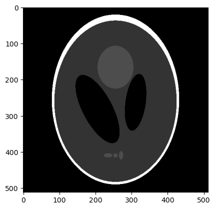
We get the ground truth image from tomopy, but this can be replaced by any image.

im_size = 512
shepp = tomopy.shepp2d(im_size)[0].astype(np.float32)/255
plt.imshow(shepp, cmap="gray")

<matplotlib.image.AxesImage at 0x7fdda79b31c0>

Simulation

First we model the ridig motion using an AffineWarpingOperator2D. \(x_1\) represents the image during subscan 1 and \(x_2\) represents the image during subscan 2. \(x\) is the dynamic image: a stack of (in this case) two images, displaying the motion:

\[\begin{split}x = \begin{bmatrix} x_1 \\ x_2 \end{bmatrix} = \begin{bmatrix} I \\ M(\theta, t) \end{bmatrix}x_1\end{split}\]

This model, expressed with a block matrix, can be programmed completely matrix free, using the matrix free warping operator and pylops.VStack to creat the block operator:

true_trans = [50, -20]
true_rot = 0.3

I = pylops.Identity(im_size**2, dtype=np.dtype('float32'))
M_2 = lambda rot, trans: imwip.AffineWarpingOperator2D(
    (im_size, im_size),
    rotation=rot,
    translation=trans,
    adjoint_type="inverse")

M = lambda rot, trans: pylops.VStack([I,
                                      M_2(rot, trans)])

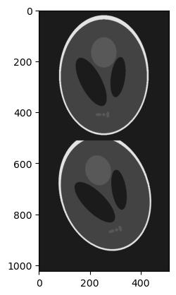
Now we can apply this model to the static ground truth image to obtain the dynamic ground truth, which we call true_x here:

true_x = M(true_rot, true_trans) @ shepp.ravel()
plt.imshow(true_x.reshape(-1, im_size), cmap="gray")

<matplotlib.image.AxesImage at 0x7fdda7823610>

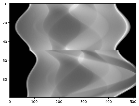
The CT system can also be expressed with matrix free operators, using the ASTRA-toolbox. A system with two subscans looks like this:

vol_geom = astra.create_vol_geom(im_size, im_size)

angles_1 = np.linspace(0, np.pi, 100)[0::2]
angles_2 = np.linspace(0, np.pi, 100)[1::2]

proj_geom_1 = astra.create_proj_geom('parallel', 1, im_size, angles_1)
proj_id_1 = astra.create_projector('cuda', proj_geom_1, vol_geom)

proj_geom_2 = astra.create_proj_geom('parallel', 1, im_size, angles_2)
proj_id_2 = astra.create_projector('cuda', proj_geom_2, vol_geom)

The full dynamic CT system becomes

\[\begin{split}\begin{bmatrix} W_1 & 0\\ 0 & W_2 \end{bmatrix} \begin{bmatrix} I \\ M_2(\theta, t) \end{bmatrix}x_1 = \begin{bmatrix} p_1 \\ p_2 \end{bmatrix}\end{split}\]

or in short

\[WM(\theta, t)x_1=p\]

W_1 = astra.OpTomo(proj_id_1)
W_2 = astra.OpTomo(proj_id_2)
W = pylops.BlockDiag([W_1,
                           W_2])

p = W @ M(true_rot, true_trans) @ shepp.ravel()
plt.imshow(p.reshape(-1, im_size), cmap="gray")
plt.axis('auto')

(-0.5, 511.5, 99.5, -0.5)

Solving

We can solve $ WM(\theta, t)x=p $ simultaniously for \(\theta, t\) and \(x\) by minimizing

\[f(\theta, t, x) = \frac{1}{2}\lVert WM(\theta, t)x-p \rVert^2\]

# objective function
def f(x, rot, trans):
    rot = rot[0]
    res = W @ (M(rot, trans) @ x) - p
    return 1/2 * np.dot(res, res)

More important for the solver is the gradient of this objective function:

\[\begin{split}\begin{aligned} \nabla_{\theta, t} f(\theta, t, x) &= \left(\frac{d}{d(\theta, t)} M(\theta, t)x\right)^T&W^T(WM(\theta, t)x-p)\\ \nabla_x f(\theta, t, x) &= M(\theta, t)^T&W^T(WM(\theta, t)x-p) \end{aligned}\end{split}\]

# gradient of objective function
def grad_f(x, rot, trans):
    rot = rot[0]

    WTres = W.T @ (W @ (M(rot, trans) @ x) - p)

    grad_rot, grad_trans = imwip.diff(M(rot, trans), x, to=["rot", "trans"])
    grad_rot = grad_rot.T @ WTres
    grad_trans = grad_trans.T @WTres

    grad_x = M(rot, trans).T @ WTres

    return grad_x, grad_rot, grad_trans

# initial guess: zero
rot0 = [0.0]
trans0 = [0.0, 0.0]
x0 = np.zeros(im_size**2, dtype=np.float32)

# solve
x, rot, trans = imwip.split_barzilai_borwein(
    grad_f,
    x0=(x0, rot0, trans0),
    bounds=((0, 1), None, None),
    max_iter=200,
    verbose=True)

100%|█████████████████████████████████████████| 200/200 [00:02<00:00, 70.74it/s]

print("estimated rotation:", rot)
print("true rotation:", true_rot)
print()
print("estimated translation:", trans)
print("true translation:", true_trans)

estimated rotation: [0.2991741]
true rotation: 0.3

estimated translation: [ 50.00546389 -19.93486514]
true translation: [50, -20]

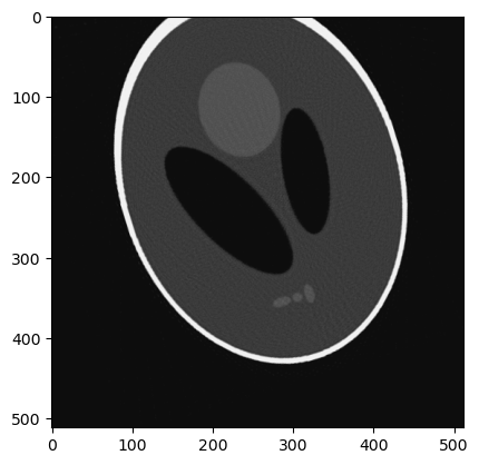
Solution in first subscan:

plt.imshow(x.reshape((-1, im_size)), cmap="gray")

<matplotlib.image.AxesImage at 0x7fdda0322d40>

Solution in second subscan

plt.imshow((M_2(rot[0], trans) @ x).reshape((-1, im_size)), cmap="gray")

<matplotlib.image.AxesImage at 0x7fdda038f9d0>